We do not collect user personal data, but we might use analytics cookies to enhance user experience and
analyze traffic.For more information, please contact us here.
An Exhaustive Guide to Decision Trees in Machine Learning
Decision Trees are a powerful and intuitive tool in machine learning, used for both classification and
regression tasks. They mimic human decision-making by breaking down complex decisions into simpler, smaller
parts through a series of binary questions. Starting from a root node, the model makes splits based on
feature values, working down branches to reach a leaf node, which provides the final prediction. Their
simplicity, interpretability, and ability to handle both numerical and categorical data make decision trees
a foundational model in machine learning, widely used across industries for solving diverse problems.
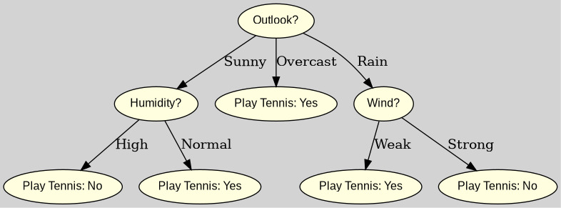
A visualization of a Decision Tree Example used in a classification task.
Now that we’ve introduced the core idea behind Decision Trees, let’s dive deeper into their structure, how
they work, and the key algorithms that power them.
A Decision Tree is a supervised machine learning algorithm used for both classification and
regression tasks. It predicts the value of a target variable by learning decision rules inferred from the input
features. The structure of a decision tree resembles a flowchart-like model, where:
Each internal node represents a decision or test on a feature. For example, it could check
if a feature value is greater than or less than a threshold.
Each branch stemming from an internal node corresponds to an outcome of the decision,
leading to the next decision or final result.
Each leaf node represents the final prediction, either a specific class label (in
classification) or a continuous value (in regression).
In essence, a decision tree partitions the dataset into subsets based on feature values, progressively honing in
on the target variable. The algorithm continues to split the data at each node until it reaches the most optimal
classification or regression output. This tree-based approach makes decision trees easy to interpret and
visualize, which is why they are widely used in practical applications.
Key concepts that help define the structure of decision trees include:
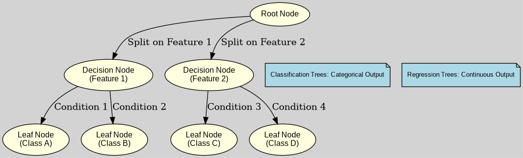
Root Node: The topmost node in a decision tree that represents the entire dataset. This is
where the first split is made based on the most significant feature that provides the highest information
gain.
Decision Node: Internal nodes where decisions are made based on features. These nodes
branch out according to the outcomes of the decision or test applied to a feature. Each branch represents a
possible value or range for the feature being evaluated.
Leaf Node: The terminal nodes of the tree, which represent the final output or prediction.
For classification tasks, each leaf node is associated with a class label, while for regression tasks, it
holds a continuous value.
Entropy: Entropy is a measure of impurity or disorder in the dataset. In the context of
decision trees, it quantifies how mixed the classes are in the data. A node with higher entropy means more
uncertainty in classification, while a node with lower entropy indicates purer (more homogeneous) data.
Information Gain: Information gain represents the reduction in entropy after splitting a
dataset based on a feature. It measures the effectiveness of a feature in improving the purity of the
splits. A feature that results in a large reduction in entropy has a high information gain and is considered
a better feature for splitting the data.
By using these concepts, a decision tree systematically partitions the data, making decisions at each node,
until it reaches a point where no further splitting is necessary, yielding the final prediction.
There are two main types of decision trees based on the target variable:
Classification Trees: They are employed when the target variable is categorical, meaning
the model is designed to predict a discrete class label. The tree splits the data based on features to
classify it into predefined categories. For example, a classification tree could be used to determine
whether an email is spam or not.
Regression Trees: They are used when the target variable is continuous. Instead of
predicting categories, these trees predict numerical values. The model works by splitting the data into
regions that minimize variance, ultimately providing a continuous output. For example, a regression tree
might be used to predict the price of a house based on its features like size, location, and number of
bedrooms.
Key concepts in the structure of a decision tree.
2. How Decision Trees Work
Here's a breakdown of how decision trees work:
Start at the root node and evaluate each feature.
Select the best feature to split based on criteria like Gini Impurity or Entropy.
Recursively split the data until stopping conditions are met (e.g., depth limit or pure node).
Impurity measures quantify how mixed or impure a set of samples is with respect to the target variable. The
common impurity measures used are Gini Impurity and Entropy.
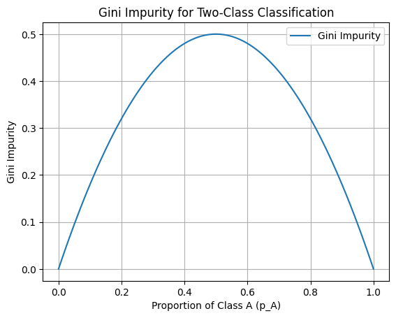
Gini Impurity
Gini impurity is a measure of how often a randomly chosen element from the set would be incorrectly labeled if
it was randomly labeled according to the distribution of labels in the subset. It is defined as:
\[
\text{Gini}(D) = 1 - \sum_{i=1}^{C} p_i^2
\]
Where:
\( D \) is the dataset,
\( C \) is the number of classes,
\( p_i \) is the proportion of instances of class \( i \) in the dataset.
A Gini impurity of 0 indicates perfect purity (all instances belong to a single class), while a Gini impurity of
0.5 indicates maximum impurity (equal distribution of classes).
Let's use a simpler two-class example to better illustrate how Gini impurity works. We'll take a dataset where
we have two classes:
Class A (e.g., "Apples")
Class B (e.g., "Bananas")
Here’s how you can visualize Gini impurity for a two-class scenario:
Gini Impurity for a two-class scenario.
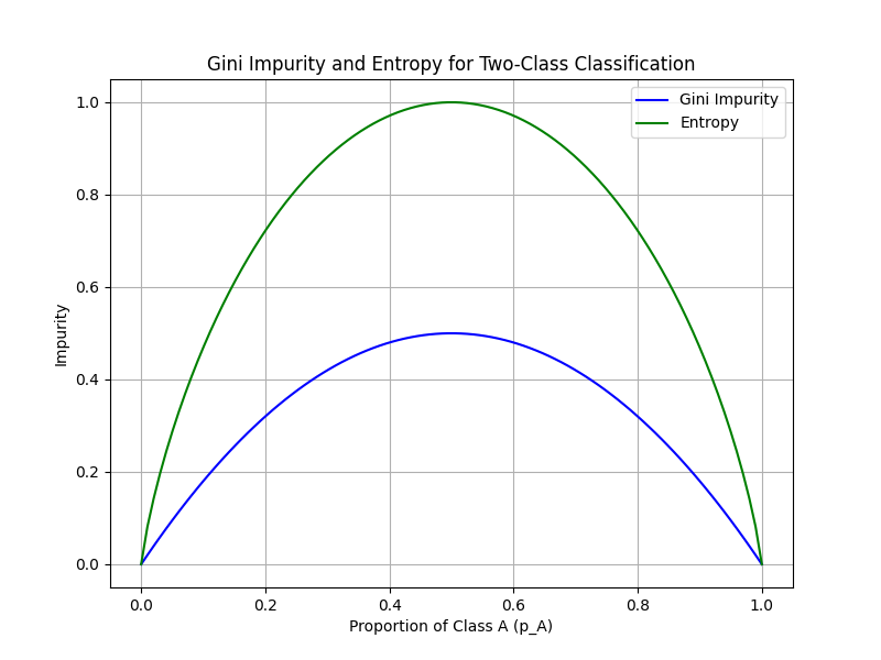
Entropy:
Entropy measures the amount of uncertainty or disorder in a set. It is defined as:
\[
H(D) = -\sum_{i=1}^{C} p_i \log_2(p_i)
\]
Where:
\( H(D) \) is the entropy of dataset \( D \),
\( p_i \) is the proportion of instances belonging to class \( i \).
Similar to Gini impurity, an entropy of 0 indicates that all instances belong to a single class, while higher
entropy indicates greater uncertainty.
Here's how you can visualize entropy for a two-class scenario:
Comparison of Gini Impurity and Entropy for a two-class scenario.
Information Gain
Information Gain is a criterion used to determine which feature to split on at each node. It
measures how much information a feature provides about the class labels. The information gain for a feature \( A
\) is
calculated as follows:
To avoid overfitting, decision trees also employ stopping criteria that can be defined mathematically, such as:
Maximum Depth: A maximum number of levels allowed in the tree.
Minimum Samples at Leaf: A minimum number of samples required to create a leaf node.
Minimum Impurity Decrease: A threshold below which further splits are not made.
Pruning
Decision trees can overfit the training data, especially when they grow deep. To prevent this, pruning methods
are applied:
Pre-Pruning (Early Stopping): Pre-pruning, or early stopping, halts the growth of the tree
before it becomes too complex. This can be done by setting constraints like:
Maximum depth: Limiting how deep the tree can grow to prevent overfitting.
Minimum samples per leaf: Specifying a minimum number of data points required to
form a leaf node.
Minimum information gain: Stopping a split if the reduction in Gini impurity or
entropy is too small, preventing unnecessary complexity.
Pre-pruning stops tree growth early but risks underfitting, as important patterns might be missed.
Post-Pruning (Pruning After Training): Post-pruning is applied after the tree has been
fully grown. The tree is allowed to reach maximum complexity, and then less important nodes or branches are
pruned. Common methods include:
Cost Complexity Pruning: A balance is struck between the complexity of the tree and
its accuracy by assigning a penalty for larger trees. Nodes are pruned if their removal does not
significantly decrease accuracy.
This method finds a subtree that minimizes the cost-complexity
function:
\[
C_{\alpha}(T) = R(T) + \alpha |\tilde{T}|
\]
Where:
\( C_{\alpha}(T) \) is the cost complexity of the tree \( T \),
\( R(T) \) is the total misclassification rate of the tree,
\( \alpha \) is a complexity parameter that penalizes the number of leaf nodes,
\( |\tilde{T}| \) is the number of leaf nodes in the tree.
Post-pruning often provides better results as it allows the model to learn the data fully and then removes
unnecessary complexity.
3. Advantages and Limitations
Advantages:
Easy to interpret and understand: Gini impurity and entropy-based models (such as
those used in decision trees) are intuitive and straightforward. The calculations involved in determining
the impurity of a split are simple, which makes it easier to understand the resulting model. Users can
easily interpret how the model works by following the conditions at each split and how the decision rules
are formed.
Works with both categorical and numerical features: Gini impurity and entropy can be used
with datasets that have either categorical or numerical features. This flexibility is particularly useful in
practical machine learning problems, where data types vary. In the case of categorical data, Gini impurity
or entropy can measure the "purity" of different categories in a node, while for numerical data, thresholds
are found to split continuous variables effectively.
Requires little data preparation: Minimal data preprocessing is required when using Gini
impurity and entropy. These measures handle raw data well, meaning you typically do not need to normalize or
scale features beforehand. The methods are robust to missing values or different units of measurement.
Additionally, both measures naturally handle multi-class data without requiring any special treatment,
unlike some other algorithms which require one-vs-rest transformations.
Limitations:
Prone to overfitting, especially with deep trees: When Gini impurity or entropy are used in
decision trees, a model can become overly complex and fit the training data too well (overfitting). This
occurs because a deep tree can keep splitting the data until each node has very few data points or becomes
"pure," which reduces generalization to new, unseen data. In practice, this means the model will perform
well on the training set but may struggle to perform well on new data.
Sensitive to small changes in the dataset: Both Gini impurity and entropy-based models are
highly sensitive to small changes in the dataset. A slight modification, such as adding or removing a few
data points, can lead to significantly different tree structures. This sensitivity can make models unstable
and less robust, meaning results can vary between runs unless steps are taken to stabilize the model, such
as pruning, limiting tree depth, or using ensemble methods like random forests.
4. Decision Trees in Python (Example)
Here’s a simple example of implementing a decision tree using Python:
from sklearn.datasets import load_iris
from sklearn.model_selection import train_test_split
from sklearn.tree import DecisionTreeClassifier
from sklearn import tree
import matplotlib.pyplot as plt

# Load the Iris dataset
iris = load_iris()
X, y = iris.data, iris.target

# Split data into training and testing sets
X_train, X_test, y_train, y_test = train_test_split(X, y, test_size=0.3, random_state=42)

# Create a Decision Tree classifier
clf = DecisionTreeClassifier(max_depth=3)

# Train the classifier
clf.fit(X_train, y_train)

# Evaluate the classifier
accuracy = clf.score(X_test, y_test)
print(f"Accuracy: {accuracy * 100:.2f}%")

# Visualize the Decision Tree
plt.figure(figsize=(12, 8))
tree.plot_tree(clf, filled=True, feature_names=iris.feature_names, class_names=iris.target_names)
plt.show()
This Python example demonstrates training a decision tree on the Iris dataset, evaluating its accuracy, and
visualizing the tree structure.
5. Common Applications
Customer Segmentation: Decision trees and classification models are frequently used in
marketing to group customers based on their behavior, purchasing patterns, or demographic characteristics.
By analyzing past behavior, businesses can create targeted marketing campaigns or personalized offers,
enhancing customer satisfaction and increasing sales.
Medical Diagnosis: In healthcare, machine learning models like decision trees can assist in
diagnosing diseases. By analyzing a patient's symptoms, medical history, and test results, these models can
help classify patients into risk groups or suggest possible conditions, supporting doctors in making more
accurate diagnoses.
Credit Risk Analysis: Financial institutions use these models to predict the likelihood of
a borrower defaulting on a loan. By analyzing factors such as income, credit history, and debt-to-income
ratio, credit risk analysis helps lenders decide whether to approve a loan and what interest rate to offer.
This improves risk management in banking and financial services.
Image Recognition: In computer vision tasks, decision trees are often combined with other
techniques like random forests or convolutional neural networks (CNNs) to classify images. For example, they
can help in identifying objects in images, detecting patterns, or recognizing facial features, which has
applications in security, autonomous vehicles, and social media platforms.
6. Frequently Asked Questions
Q1: When should I use decision trees over other algorithms?
Use decision trees when you need a model that is easy to interpret and when your dataset has both categorical and
numerical features.
Q2: How can I prevent overfitting in decision trees?
Overfitting can be reduced by applying pruning techniques or adjusting hyperparameters like
max_depth and min_samples_split.
Q3: What is the difference between Random Forests and Decision Trees?
A decision tree is a single model, while a Random Forest is an ensemble of multiple decision trees that combine
their predictions to improve accuracy.
Q4: Can decision trees handle missing values?
Yes, decision trees can handle missing values by using surrogate splits or by treating missing values as a
separate category.
Q5: Are decision trees sensitive to the data used for training?
Yes, decision trees are sensitive to training data; small changes can lead to different tree structures, making
them unstable.
Q6: How do decision trees handle categorical variables?
Decision trees can directly work with categorical variables by splitting on the categories without needing to
convert them into numerical form.
Q7: What are some common applications of decision trees?
Decision trees are commonly used for customer segmentation, medical diagnosis, credit risk analysis, and image
recognition.